Update functions
| « PREV | NEXT » |
The moment we’ve all been waiting for…
Up to this point, we have implemented some effects that were visually impressive eye candy, but were otherwise ambient and didn’t have much influence on the world around them. Starting from this chapter, we will be implementing particles that exhibit complex, dynamic behavior and can have tangible effects on the game itself, beyond just the graphical qualities they provide. Particles, which can be characterized by reactivity and/or interactivity (with Lara, other entities, the room geometry or the game engine / TRNG itself). This is made possible thanks to update functions, which allow to define the collective behavior a group of particles will exhibit. This mechanism permits the particles to act in a user-defined way and have unique, scriptable attributes (such as colliding with the environment, setting Lara on fire, doing damage on contact with an enemy, homing onto a target, etc).
More than anything else, it is this ability to code custom behavior which sets apart the particles offered by this plugin from the particles you have seen before, in FLEP or the vanilla engine. The incredible flexibility provided by update functions in tandem with the various helpful API functions allows one to script things ranging from new traps, new weapons and attacks for both Lara and her foes, magical abilities, unique puzzles, never seen before gameplay mechanics, the list goes on. This feature is very powerful, but as we all know, “with great power comes great responsibility”. It can easily lead to some disastrous results (including but not limited to: crashing the game) if you are not being cautious, so tread carefully!
In the first section of this new chapter, we will return to the previously neglected update function of the dust effect back from Chapter 1. This time around, I’ll give a proper explanation of update functions and how to write a simple one that makes the particles animate over their sprites. Afterwards, we will learn of the t-parameter property of particles, which allows to correlate a particle’s age with another property through some mathematical formula. A specific example of this will be given in the section on shaping particle trajectories. We will subsequently utilize the t-parameter in context of explaining how the sizeCust and colCust override fields work.
Similarly to Chapter 1, this chapter is also split int
Sections
1. Update functions
2. How update functions work
3. Writing a simple update function
4. Stochastic particle motion
5. Particle t-parameter
6. Shaping particle trajectories
7. Particle sizeCust and colCust
2. How update functions work
3. Writing a simple update function
4. Stochastic particle motion
5. Particle t-parameter
6. Shaping particle trajectories
7. Particle sizeCust and colCust
Update functions, for real this time
Back in Chapter 1, when we created our dust particle effect, we started writing an update function for it. However, we quickly abandoned it when it became apparent that we won’t need it for our relatively simple dust effect.Don’t worry, we will be bringing that poor little update function back from oblivion now! Let’s recall the entire dust.lua module script, including the (commented out) dustUpdate() function:
			    local dustgroup


			    local function dustInit()

			        local part = createSpritePart(dustgroup) -- create a sprite particle of the "dust" group


			        part.emitterIndex = getTombIndex(12) -- get tomb4 item index of item with NG index 12


			        part.lifeSpan = 30 * 4 -- 30 frames * 4 = 4 seconds

			        part.sizeStart = randomInt(150, 300)

			        part.sizeEnd = part.sizeStart * 3 -- make dust slowly expand over time


			        part.colStart.r = randomInt(130, 150)

			        part.colStart.g = randomInt(100, 120)

			        part.colStart.b = randomInt(70, 85)

			        part.colEnd = part.colStart


			        -- randomize position

			        local dx = randomFloat(-512, 512)

			        local dy = randomFloat(-512, 512)

			        local dz = randomFloat(-512, 512)


			        -- since we assigned an emitterIndex, the particle spawn position is in relation to the emitter item

			        part.pos.x = dx

			        part.pos.y = dy

			        part.pos.z = dz


			        -- randomize velocity

			        part.vel.x = randomFloat(-5, 5)

			        part.vel.y = randomFloat(-5, 5)

			        part.vel.z = randomFloat(-5, 5)


			        part.spriteIndex = 0 -- "smoke" sprite texture

			        part.fadeIn = 30 -- fade in for 1 second

			        part.fadeOut = 30 -- fade out for 1 second


			        -- randomize rot and rotVel

			        local degrees = randomInt(0, 359)

			        part.rot = degToRad(degrees)


			        local rotspeed = randomNegate(randomFloat(2, 4)) -- generate a random value between 2 and 4, negate it half of the time

			        part.rotVel = degToRad(rotspeed)

			    end


			    --[[

			    local function dustUpdate(part)

			    end

			    --]]


			    -- creation of our particle group and assigning it to the variable

			    dustgroup = createGroup(dustInit, nil) -- passing nil in place of our dustUpdate
Recovering the update function
First of all, we’ll uncomment the dustUpdate() function. We can do this either by removing the multiline comment tags or adding an extra minus / hyphen to the opening tag, ---[[ . Both ways are acceptable, but I’ll opt to simply remove the comment tags altogether. The next step is to restore dustUpdate as the second argument to createGroup(), in place of the nil value we put before:
local function dustUpdate(part)
end
-- creation of our particle group and assigning it to the variable
dustgroup = createGroup(dustInit, dustUpdate) -- restored dustUpdate as second argument
By the way, I feel like I should explain why I generally write the parentheses after the name of a function, e.g. dustUpdate(), but specifically when speaking of passing the function as an argument to a function like createGroup(), I drop the parentheses, i.e. dustUpdate.end
-- creation of our particle group and assigning it to the variable
dustgroup = createGroup(dustInit, dustUpdate) -- restored dustUpdate as second argument
This inconsistency is not by mistake or due to negligence. When I write the name of a function generally, I add the parentheses to emphasize it being a function (and not an ordinary variable with a value like 5). However, when I talk of passing a function as an argument to another function, I deliberately omit the parentheses after the name. This is because attempting to pass the function with parentheses to its name, like for example:
dustgroup = createGroup(dustInit(), dustUpdate() ) -- this is incorrect!
is improper syntax in Lua. In the above snippet, we are no longer passing the dustInit() and dustUpdate() functions as arguments, but rather calling each function without any arguments, then passing the values returned by these functions (or rather lack thereof, since neither should return anything) as the actual arguments passed to createGroup(). If the functions were to return something, like a number, we would be passing that returned number as an argument to createGroup() (and since this is not what createGroup() is expecting to receive as arguments, the plugin would raise an ERROR). However, if the functions do not return anything (as is in our case), it is the same as passing nil instead of the function. Effectively, the createGroup() call turns into createGroup(nil, nil). This results in the same problem we had by not respecting the correct order of the code back in Chapter 1, if you remember – a group with no init and no update function assigned, preventing any particles from spawning for this group.If the reason for dropping the parentheses is still not clear to you, it may help to consider another perspective. Remember when I said that function names are actually just disguised variables? This means that the variable is storing a value. What value would that be? The definition of some function (this is an oversimplification, but assume that’s what you get when you ask for a function variable’s “value”). When we want to pass a Lua function as an argument, we want to pass its value (the definition) – not its returned result. So, we are treating it as we would any other variable that holds a value. To pass the value from a variable as an argument, we never used parentheses, right? For this logic of no parentheses to be consistent, we are thinking of dustInit and dustUpdate not as functions, but as variables, containing some value we want to pass.
To emphasize the difference between calling functions and passing them as arguments, I will omit the parentheses to indicate that a function will not be called, but rather passed as an argument to another function (i.e. treated as a variable with a value). In all other cases, I’ll refer to the function with parentheses attached to its name, emphasizing that it is, indeed, a function to be called in the script.
How update functions work
Coming back to our group definition, we are now constructing our group with both an init and an update function. Of course, our update function is not doing anything at the moment. We will make it do something soon, don’t worry, but before we can proceed, we should first be capable of answer the following – what are update functions, exactly, and how do they work?I already mentioned before that the update function expects a single argument, a particle instance from the group. The function argument’s name becomes an alias for the particle instance it is currently working on. We can choose whatever alias we want, really, but in these tutorials, we always use the name part, as per our convention.
But wait, – you might ask – doesn’t that go against the rule of not using an identical name for another variable in the script? After all, we’ve already used part as the name for the newly created particle instance in the dustInit() function…
Fret not, in this case it doesn’t matter the names are identical. The reason why it’s okay to used the name part in both the dustInit() and dustUpdate() functions is because these are, in fact, two unrelated variables. Both are enclosed within the code blocks of their respective functions (one being the init, the other being the update function). They are not in an outer scope of the script, like the dustgroup variable, for example. If we were to use the part name somewhere in the outer scope, outside of all functions, if blocks and for loops, then reuse the name a second time inside the init or update function, then indeed we would be dealing with a name collision and could run into potential problems of ambiguity.
But in our case, the part variables are occupying two different locations in the code and Lua is smart enough to recognize that these are not the same, but completely distinct variables, that just happen to use the same name in their respective scopes (one scope is the init function block, the other scope is the update function block). If you want to be extra careful though, you may of course use a different name for the part alias in the update function. Just use another short one for your own sake, unless you love typing a lot.
Particle System Update Loop
Anyway, what purpose does the argument part serve to dustUpdate()? Simply put, part is one of the particle instances belonging to the particle group. During each in-game frame, the particle system iterates through all currently active (alive) particles. It performs generic updates to each of those particles (like updating their positions or decreasing their life counters). On top of that, it calls the update Lua functions we assigned to particle groups (unless nil was used in their place that is), dispatching all the particle instances belonging to a certain group to the corresponding update function, through the part argument (serving as the alias of the given particle instance inside the update function). This is the Particle System Update Loop: Given that update is called for every active particle in the group, part becomes the alias of the specific particle instance on which the update function was currently called (as the plugin moves through the sequence of all exisiting particles in the current cycle of the game loop). This way, every particle in the group has the opportunity to be modified by the designated update function assigned to the group, on each game cycle. In our update function, through the part alias, we have access to the particle’s properties, including all of the properties we have talked about so far, and a few we have not mentioned yet. We can then inspect or change the particles’ positions, velocities, rotations, sizes, colors, so on and so forth, to our own will and liking!
Okay, enough of the exposition, already. Time to make the update function actually do something with our particles!
Writing a simple update function
How about this – for testing purposes, on each successive tick, we make the particles jump to the next sprite texture in DEFAULT_SPRITES. They will start out with part.spriteIndex = 0 in the init function, then keep iterating through the different textures from DEFAULT_SPRITES in the update. Sounds simple enough, right?The update function for that may look something like this:
local function dustUpdate(part)
part.spriteIndex = part.spriteIndex + 1
end
Nothing too sophisticated, as you see. We are taking the current value of part.spriteIndex, adding 1 and assigning this new value back to spriteIndex. Easy, right?part.spriteIndex = part.spriteIndex + 1
end
Let’s run the game and see what we have. We launch the level and…
Indeed, all of the particles animate through the sprite textures, but only once, then they stop at the last texture of DEFAULT_SPRITES! Not only that, but if we enable the console logger to see what’s going on behind the scenes, we see we’re being bombarded with WARN messages:
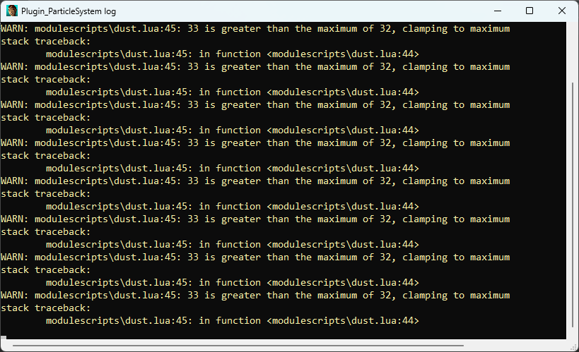
Don’t worry, we can fix this. We have just blundered with the above code for increasing the part.spriteIndex, that’s all. To understand why this doesn’t work correctly, let’s inspect the DEFAULT_SPRITES object in either WadTool, WADMerger’s sprite editor or the Sprite Tool in NG Center (on the first Tools tab). If you are using an unmodified DEFAULT_SPRITES, we can see that there are 33 textures contained inside of it, indexed 0 to 32.
The particles first are assigned texture 0, as we indicated in the init function (part.spriteIndex = 0). The update function makes part.spriteIndex move to texture 1, then 2, then 3… if we continue this pattern, we eventually reach the last texture at index 32. What happens during the update at that point? The part.spriteIndex should increase to 33, but… there is no texture with that index number in the DEFAULT_SPRITES! This situation, if left unmanaged, would result in a nasty crash, since the Tomb4 engine would not know how to handle it. However, as we have just seen, instead of crashing the game, the particles simply stop updating their texture upon reaching the final one.
Why is there no crash, then? This is a protective measure within the plugin. To ensure that such a nasty crash never occurs, if the part.spriteIndex goes beyond the number of existing sprite textures, the plugin sets it back to the highest possible texture index in the sprite slot (32 in this case) and sends a warning message in the logger. Consider this a kind gesture from the plugin developers… ;)
How to fix this
You probably don’t want the particle to animate only a single time and then stop, it would be better if this animation would repeat over and over again! Since the number of textures in (unmodified) DEFAULT_SPRITES is 33 and we want the update function to keep going through all the indices 0-32 in a loop, but never go above 32, there is a specific arithmetic operator that solves this exact problem. Do you remember which one? I hope you had the modulo operator % in mind. If you did not, then… nothing, just remember it is very convenient for these types of situations!We will use the total number of sprite textures in DEFAULT_SPRITES (by default, 33) as the modulo, on the incremented spriteIndex. This will make the spriteIndex continuously cycle between integers 0-32, exactly what we want. We first need to put the expression part.spriteIndex + 1 in parentheses. According to the PEMDAS rule, when an operation is inside parentheses, that calculation is performed first. We do this because we want to ensure addition is done before the modulo operation, otherwise the order would be part.spriteIndex + (1 % 33), which is not what we want. After the closing parenthesis we place the modulo operator % with 33 on the righthand side:
local function dustUpdate(part)
part.spriteIndex = (part.spriteIndex + 1) % 33
end
Let’s try running it in game again.part.spriteIndex = (part.spriteIndex + 1) % 33
end
Problem averted! Though the aesthetic quality of such particles is… questionable, we see they loop flawlessly through all of the textures in DEFAULT_SPRITES.
You can certainly use this approach to make particles animate through a looping sprite sequence (and not a bunch of unrelated sprites as in our example). However, in the second half of this chapter, I’ll demonstrate a function named partAnimate() which does this for us and allows to set both the exact texture range and the framerate for this animation. Way more convenient than doing it ourselves!
Stochastic particle motion
The title of this section probably sounds scary, but I’m just using big words to sound smart. The subject matter is really trivial, as you will see.The goal for this section is using an update function to make particles move in a random, unpredictable pattern (stochastic is just a fancy word for “random”, in case you didn’t know), rather than in some constant, unchanging direction defined in the init function. In doing so, we can simulate several organic effects, like that of molecules dispersing in air or liquid, or less abstractly, a cloud of insects or other creatures flying off in various directions. Sounds fun, right?
We’ll first set up a particle group with an init function that will generate some colorful particles around Lara:
					local molecules


					local function moleculeInit()

					    local part = createSpritePart(molecules)


					    part.emitterIndex = getLaraIndex()

					    part.emitterNode = 0 -- hip mesh


					    part.lifeSpan = 60

					    part.fadeIn = 20

					    part.fadeOut = 20


					    part.spriteIndex = 14


					    part.sizeStart = randomInt(40, 80)

					    part.sizeEnd = part.sizeStart


					    part.colStart.r = randomInt(0, 255)

					    part.colStart.g = randomInt(0, 255)

					    part.colStart.b = randomInt(0, 255)


					    part.pos.x = randomFloat(-512, 512)

					    part.pos.y = randomFloat(-512, 512)

					    part.pos.z = randomFloat(-512, 512)

					end


					local function moleculeUpdate(part)

					end


					molecules = createGroup(moleculeInit, moleculeUpdate)
The first attempt at randomized motion
We have to now think about how we may go about simulating random motion on particles. By “random”, I mean that it should be impossible to predict where any individual particle will travel, it will be determined by a random process. What if we applied a randomized velocity on X, Y, Z, on each game tick, through the update function?
local function moleculeUpdate(part)
part.vel.x = randomFloat(-50, 50)
part.vel.y = randomFloat(-50, 50)
part.vel.z = randomFloat(-50, 50)
end
What kind of result does this give us? Let’s see!part.vel.x = randomFloat(-50, 50)
part.vel.y = randomFloat(-50, 50)
part.vel.z = randomFloat(-50, 50)
end
Well… it’s random alright! This probably looks fine for something like gas molecules, but such movement is too jittery to be seem organic, like living insects…
To understand why our particles are jittering, let’s think about what happens on each tick, with a line such as:
part.vel.x = randomFloat(-50, 50)
If we had this line inside the init function, the generation of the X velocity value would happen only once, at particle spawn. However, we have this line inside the update function, which changes things. The X velocity in the field part.vel.x recieves a random number generated from randomFloat(-50, 50) on each consecutive tick during the particle’s lifetime. We know that velocity conveys the immediate change (i.e. “jump”) in the particle’s position, on each tick. But remember what I told you when I first introduced these random functions? They always generate a new random value on each successive call. This means that a potential sequence of these values could look like:
47.054, -31.496, 1.032, -13.354, -2.822, 48.026, -5.659, -46.55, 27.086, -4.082, -37.156, -18.964, 2.69, -1.446, 5.916, -45.484, 39.806, -27.617
Now, let’s make a simple plot, displaying these random velocity values obtained during each tick: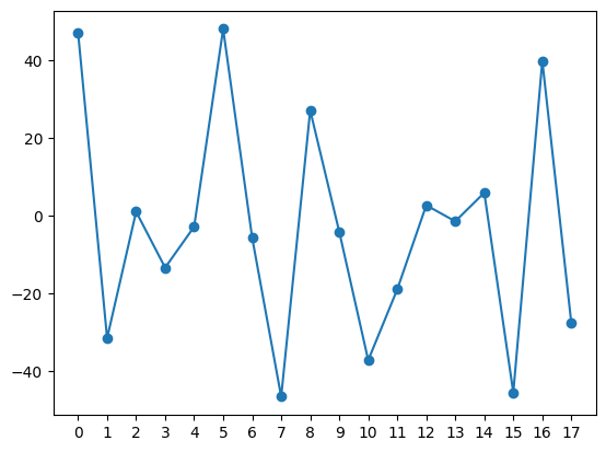
Do you see the problem? there is no smooth, cohesive pattern between the value obtained on one tick and the tick after. This means that the changes to position on each (X, Y, Z) axis manifest as abrupt “jerks” in the particle. This jittering effect only gets worse with larger random ranges on velocity. In my truest fashion, I will now tell you there is a special method of generating random(ish) numbers which are “random, yet smooth” and thus do not have this jittering problem when used on velocity. However, we shall cover this mysterious technique – yup, you guessed it – in a later chapter (“our princess is in another castle”, after all).
The second attempt – using acceleration
For now though, we can do something else. We are applying the random values directly to velocity, which conveys an immediate change in position. What if we took a step backwards and applied this randomness to acceleration, the change in velocity, instead?
local function moleculeUpdate(part)
part.accel.x = randomFloat(-10, 10)
part.accel.y = randomFloat(-10, 10)
part.accel.z = randomFloat(-10, 10)
end
If we test this in game, we see:part.accel.x = randomFloat(-10, 10)
part.accel.y = randomFloat(-10, 10)
part.accel.z = randomFloat(-10, 10)
end
that the particles quickly fly off in random directions! But we’re onto something here, because the motion itself appears a lot smoother now. Our particles do eventually pick up more speed, though, as the velocity accumulates. Now, if we could only keep the particles at bay, somehow.
Remember when we talked about enacting a fake “friction” force on particles with acceleration? I said that when the particle velocity changes dynamically over the course of the particle’s life, we must apply a different technique, applicable in update functions. So, let’s learn about it now!
The idea is incredibly simple. On each tick, the particle’s current velocity on each axis gets multiplied by a constant smaller than 1.0, and this gets assigned back to the velocity for the given axis:
part.vel.x = part.vel.x * 0.9
part.vel.y = part.vel.y * 0.9
part.vel.z = part.vel.z * 0.9
We can also take advantage of vector arithmetic – if the scaling factor on each axis is identical, the shorthand equivalent to the above is:
part.vel.y = part.vel.y * 0.9
part.vel.z = part.vel.z * 0.9
part.vel = part.vel * 0.9
What is happening in either of the above snippets is that we effectively reduce the velocity by a small percentage (fraction). Now, the percentage that remains can be large, like 90% (0.9) or even 99% (0.99), but it’s nonetheless a fraction of the whole value. What effect will this have over the course of many ticks? Well, it will ever so slightly keep nudging the particle speed down to zero, on every tick. If the particle velocity never changed (i.e. it was assigned only once in the init function), we would have another “slowdown” effect, where the particle speed would approach zero. However, in the case of our particles, we additionally have an opposing effect at play: the randomized acceleration burst!
local function moleculeUpdate(part)
part.accel.x = randomFloat(-10, 10)
part.accel.y = randomFloat(-10, 10)
part.accel.z = randomFloat(-10, 10)
part.vel = part.vel * 0.9
end
What happens when these two effects – acceleration bursts and velocity reduction – meet? Well, we get something quite interesting, see for yourself!part.accel.x = randomFloat(-10, 10)
part.accel.y = randomFloat(-10, 10)
part.accel.z = randomFloat(-10, 10)
part.vel = part.vel * 0.9
end
We see that the particles never pick up significant speeds, due to the halting effect of velocity reduction, but never completely stop moving, due to randomized burst of accelration! This mimics a form of motion that almost feels organic, like with molecules, or some living organisms dispersing through the air. The more astute of you may even recognize this pattern of motion from the party.lua module, where this exact effect was put to use.
Particle t-parameter
As you know by now, a particle has two distinct life properties. The first one, part.lifeSpan, as the name implies, describes the total amount of life the particle has. The other life property, part.lifeCounter, counts down the remaining life of the particle. In the init function, it’s implicitly assigned the same value as for part.lifeSpan, but afterwards is automatically decreased by 1 on each game cycle. Once part.lifeCounter reaches 0, the particle dies and is no longer updated or drawn by the particle system.Let’s ponder for a moment about the following. Assume we wanted to have a general way to describe a particle’s “life-stage”, regardless of its actual lifeCounter value. Something like a percentage of elapsed life. How could we do that?
Instead of using the particle’s part.lifeCounter value, which is an integer in the range [0, part.lifeSpan], we can picture a decimal (float) value between 0.0 and 1.0 (equivalent to a percentage between 0% and 100%). At 0, the particle has been newly born into the world. At 1.0 (100%), the particle reached the end of its life and ceases to exist. All in-between values describe the decimal fraction of how far a given particle is into its life course, regardless of the actual lifeSpan and lifeCounter for the given particle instance. For example, a value of 0.5 would mean that the particle is halfway through its existence (perhaps experiencing a mid-life crisis, because of it).
Jokes aside, if we have the lifeSpan and lifeCounter values, how do we calculate this “current lifestage” percentage value? It’s actually a pretty simple calculation of the form:
local lifestage = (part.lifeSpan - part.lifeCounter) / part.lifeSpan
We just subtract part.lifeCounter from total part.lifeSpan and divide the result by part.lifeSpan again. This value will always be somewhere between 0 and 1, regardless of how big or small lifeCounter and lifeSpan really are (that is, unless you tampered with the part.lifeSpan and/or part.lifeCounter values outside of init, which as yet another reminder, you should never do).Fortunately, we don’t have to carry out this calculation ourselves every time we want to use this life-percentage value for some purpose. Particles provide a special read-only property called the t-parameter, with the field name part.t (that is, a single lowercase t), which gives the 0 to 1 lifestage fraction value readily for the particle:
part.t -- read-only property, gives a 0 - 1 normalized age for the part
As mentioned, this property is read-only, which means that you can only read (copy) its current value. You cannot assign custom values to it, that results in an ERROR.How the t-parameter can be used
Okay, that’s great and all, but what would this t-parameter even be useful for? Well, picture the following situation. You would like another particle property, like its size, color or velocity, to depend on this “lifestage” value in some way. The part.t value is always in the rigid range of 0.0 to 1.0 (unlike part.lifeCounter values, which are integers and aren’t always uniform form one particle to the next, due to randomized life-spans). The t-parameter grows linearly with time (while lifeCounter values go down), reflecting the particle “progressing” its life-span. If you’re more of a visual learner, here is a graph of the t-parameter values, plotted against lifeCounter values of a particle with lifeSpan set to 100.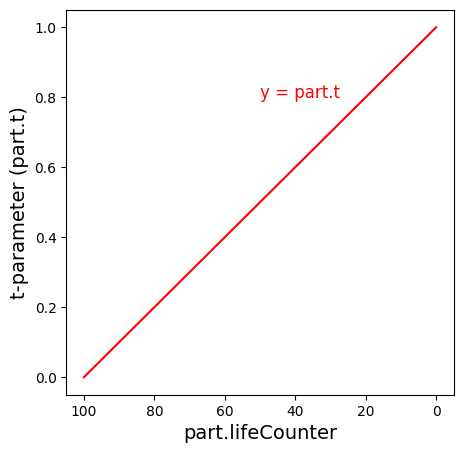
Importantly, the actual lifeSpan and lifeCounter is irrelevant here, the part.t value always moves up from 0 towards 1 (it acts like a percentage, relative to lifeSpan). Therefore, by applying some simple mathematics, you can come up with a formula that translates the 0.0 to 1.0 value of part.t to a value usable for the size, color or velocity. In slightly more mathematical terms, the t-parameter can be an input for some function, where we want some property to vary as the particle ages. This is a more generalized approach to the straightforward blending between sizeStart / sizeEnd and colStart / colEnd.
You may interject that for velocity, we already have a way to change it without using an update function – by setting an acceleration on the particle. And I say to that: okay, but what if we want the particle moving in a circular orbit? This involves a continuous change in acceleration (along with velocity and position) over time. For such cases, we can’t rely on just setting the part.accel vector a single time (in the init function) and be done with it. A circular orbit implies continuous adjustment of velocity and/or acceleration per each tick, forcing us to use an update function, there’s no way around it.
Here’s where the t-parameter can shine – since its value is guaranteed to be between [0.0, 1.0] and increases at a constant, linear rate, as the particle ages, we can create an expression that makes the velocity depend on this t-parameter in some way.
Maybe you still don’t see the full picture of how this can be useful for particle effects. Well, let’s see an example in the next section!
Shaping particle trajectories
We will now entertain a scenario in which we want the particle velocity to depend on the particle t-parameter in some way. The specifics of it are entirely up to us. We can come up with any formula that can be expressed in mathematical terms, which Lua is able understand. In doing so, we’ll utilize what we know of the t-parameter. Considering it always goes from 0 to 1 for each and every particle individually, we can perform mathematical operations on the value given by part.t to end up with a velocity that corresponds to the current life-stage of the particle.I will now ask you to reach back to your maths education in school. You most likely encountered a thing called trigonometry, do you remember? It is a discipline of maths studying how the size of angles in triangles relates to the lengths of triangles’ sides. There are two “main stars” that almost always show up when talking about trigonometry:
- the sine function – sin()
- the cosine function – cos()
If we consider a right-angled triangle (triangle with one of its angles equal to 90°), the sine function describes the length ratio of the opposite side to the hypotenuse side. The cosine function describes the ratio of the adjacent side to the hypotenuse. There is also the tangent function – tan(), describing the ratio of the opposite to the adjacent:
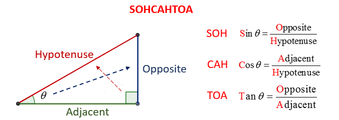
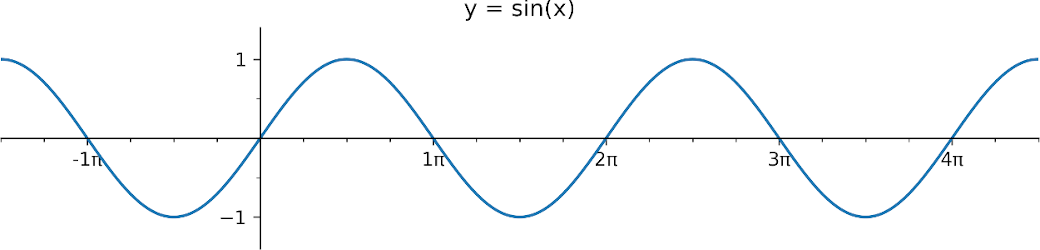
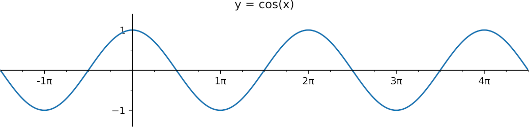
Per the above image, the angle the trigonometric functions are referencing is denoted with the lowercase greek letter θ (theta). Most commonly, the angle value of θ is expressed in radians (as a reminder, with radians, everything is based around the number π, with π/2 representing 90 degrees, π representing 180 degrees and 2π representing a full 360 degree turn). The sin() and cos() functions are continuous (without any gaps or abrupt changes) and periodic (repeating). Their specific wave-like shape repeats with an interval of 2π radians (360 degrees) and they smoothly oscillate between the output values of -1 to 1, then from 1 to -1, then back again, over and over.
Waving particles
To achieve an undulating “wave” of particles, we can give particles a Y velocity coming as an output from the sine (or cosine) function, given a certain input for the function. What should this input be? Well, the sin(x) function takes a single argument, x, which is some number value (e.g. like that of an angle). In reality, we can use any number value we want, even one that is derived from particles themselves. An obvious one worth considering in this case is part.t, of course. We will use the value of part.t as an input argument for sin(x), paired with a constant (unchanging) velocity for the other two axes, X and Z. This sounds a lot scarier than it actually is, you’ll see it’s quite simple in the code.Because the Y velocity will change over time (in a complex way, which part.accel cannot do justice), we must use an update function to achieve this.
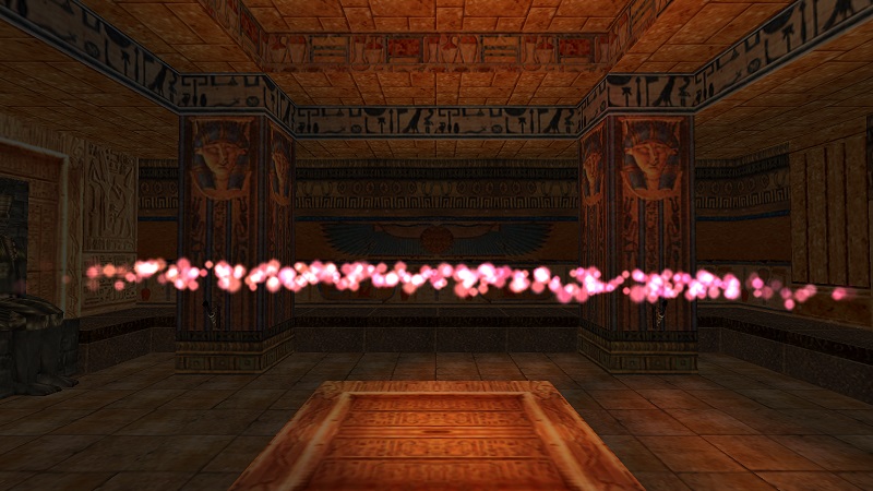
Given the below orangish-pink dot particles with a part.lifeSpan of 240 (8 seconds):
				  local wave


				  local function waveInit()

				      local part = createSpritePart(wave)


				      part.emitterIndex = getTombIndex(3) -- spawn near moveable with NGLE ID 3


				      part.lifeSpan = 240

				      part.sizeStart = randomInt(64, 128)

				      part.sizeEnd = part.sizeStart


				      part.spriteIndex = 14

				      part.fadeIn = 30

				      part.fadeOut = 30


				      part.colStart.r = 255

				      part.colStart.g = randomInt(96, 128)

				      part.colStart.b = randomInt(96, 128)


				      part.colEnd.r = randomInt(192, 255)

					    part.colEnd.g = part.colStart.g - 30

					    part.colEnd.b = part.colStart.b + 30


				      local dx = randomFloat(-512, 512)

				      local dy = randomFloat(-64, 64)

				      local dz = randomFloat(-64, 64)


				      part.pos.x = dx

				      part.pos.y = dy

				      part.pos.z = dz

				  end


					local function waveUpdate(part)

					end


					wave = createGroup(waveInit, waveUpdate)
local function waveUpdate(part)
part.vel.y = sin(part.t) -- velocity derived from the sin() function applied to part.t
part.vel.z = -20 -- constant Z velocity
-- part.vel.x defaulted to 0 from the particle init
end
As you see, in the waveUpdate() function we’re setting a Y velocity via the formula -sin(part.t) and for the Z velocity we set the constant value -20.part.vel.y = sin(part.t) -- velocity derived from the sin() function applied to part.t
part.vel.z = -20 -- constant Z velocity
-- part.vel.x defaulted to 0 from the particle init
end
We give it a run in game, and uhh…
Our particles aren’t really waving, moreso they’re moving in a rather straight line. Recall that the raw value of part.t goes from 0 to 1, directly increasing with the particle’s age. Perhaps the problem is that such a value range is simply too small for the wavy nature of sin() to become apparent? We should make it larger, in that case.
Since these trigonometric functions anticipate input values in “radian scale”, a good start would be to multiply part.t by 2π, a single interval (“wave”) of the sine function. This moves the value range of part.t from [0, 1] to [0, 2π]. By doing so, the particles should at least be able to complete a single “wave” of the sin() function. For convenience, we will make use of the built-in constant, PI_TWO (we could also use 2 * PI instead).
We’ll make the following modification for calculating the Y velocity in the waveUpdate():
part.vel.y = sin(part.t * PI_TWO)
Well… still no evident waving. Let’s remind ourselves that sin() and cos() functions return values in the [-1, 1] range, making the resulting Y velocity oscillations very insignificant. This “flattens” the shape and makes it seem almost like a straight line. Let’s turn it up a notch by multiplying the returned result by 20-30 (or something in that ballpark).
part.vel.y = sin(part.t * PI_TWO) * 20
Okay, at least now we’re able to see clear evidence of curving into a wave-like shape! But yet, there’s something off about the shape the particles trace out…
Assuming that we are looking at the traced curve as if it started out at the origin point (0, 0) on the graphs above, you may notice the shape of the curve does not match up with the graph we’d expect for sin(x), despite us using the sin() function. Come to think of it, it seems to match more closely with the cos(x) graph! No, I didn’t get the functions mixed up with one another by accident, the math is definitely correct. Something different is at play here.
The first thing we must observe is that in the TR engine, the order for the Y axis is inverted. As it goes to lower and more negative values, you go higher up in the level map (and vice-versa). That’s an easy thing to fix, we just need add a minus in front of the call to sin(), in order to negate the overall output:
part.vel.y = -sin(part.t * PI_TWO) * 20 -- Y axis is inverted so use the negative
However, this simply flips the curve upside-down (the valley becomes a peak), it does not entirely fix the shape.The other reason why it does not match up with the sin(x) graph is because we are modifying the velocity (rate of change to position) of the particles, rather than position of the particle directly. Whenever we do this, we cannot simply reuse the formula we’d use normally for position, because in the majority of cases, applying it to velocity results in something vastly different. The reasoning behind it is a mathematical concept known as calculus. This is a more advanced mathematical topic that will be touched on eventually, for more complex velocity formulas. I will not bother you with it right now though, all you need to know is because we are modifying the velocity, instead of position, we must actually use the -cos(t) function, instead of -sin(t) (although it seems arbitrary, there is concrete reasoning behind this transformation, although it requires its own, dedicated explanation, which is quite math-heavy and not our main focus). The expression for velocity should thus be changed to:
part.vel.y = -cos(part.t * PI_TWO) * 20
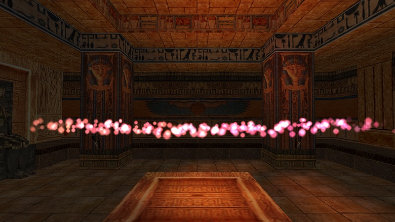
Fantastic, we finally have a nice wave of particles, following the shape of the sin(x) graph. One, single interval is a bit boring, though, so let’s squeeze in more of them in the particle “graph”. Instead of multiplying part.t by 2π, we multiply it by something bigger, like 6π (3 * PI_TWO or alternatively, 6 * PI), which should result in 3 complete intervals during each particle’s life:
part.vel.y = -cos(part.t * 3 * PI_TWO) * 30
Ah, fabulous!
Animating the wave through time
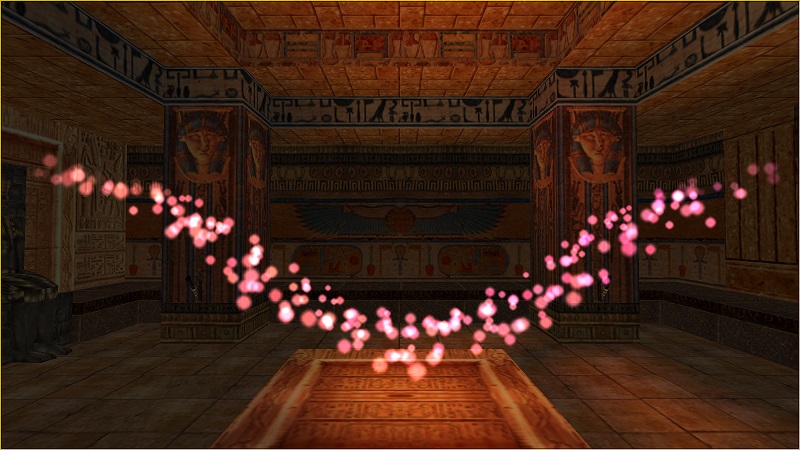
What if we go a step further and make the wave shape animate over time? It’s not that hard to achieve, we just need to add a universal time component into the expression. And by time component, I mean getGameTick() – you remember it, right?We need to somehow add this tick value to the part.t value already inside the cos() function. Unfortunately, the raw game tick value will increase way too fast to achieve a nice effect. We can first downscale it by a factor of, say, 0.002 and save this to a local time helper variable. Then add it to part.t within extra parentheses, to prioritize addition over multiplication. Finally, we multiply the whole thing by 6π, as before:
local time = getGameTick() * 0.002
part.vel.y = -cos((part.t + time) * 3 * PI_TWO) * 30
part.vel.y = -cos((part.t + time) * 3 * PI_TWO) * 30
 Voilà!
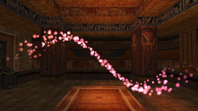
Helical trajectory
These waving particles are cool, but we can take it to the next level, by turning waves into helices or corkscrew shapes! Recall again the properties of sin() and cos(). I mentioned that these functions are phase-shifted in regards to each other. More specifically, sin(x) is π/2 radians “delayed” behind cos(x), thus cos(x) = sin(x + π/2). This phase-shift actually has a very neat origin / reason behind it. Take a look at the animated diagram below:
Allow me to explain what we’re looking at here. Let’s say we have an angle, which we will again call θ – the greek letter theta. What do we get when we use the pair of trigonometric functions, cos() and sin() on the angle θ? As it turns out, the outputs of these functions track the coordinates on the green unit circle of radius 1, centered at the origin point (0, 0). Specifically, cos θ tracks the X coordinate and sin θ tracks the Y coordinate. As the angle θ changes, cos θ (blue graph) shows how the X coordinate changes, while sin θ (red graph) shows how the Y coordinate changes on the unit circle. Observe that both of these function graphs have the same shape, but given the same input of θ, seem to be “delayed” with respect to one another. It is this specific “delayed” relationship between sin() and cos() functions that results in the (X, Y) coordinates tracing out a unit circle! Thus, each point p = (X, Y) lying on this unit circle is described by the below equations, as θ sweeps from 0 radians to 2π radians (i.e. 0° to 360°):
X = cos(theta)
Y = sin(theta)
Now, we’ll step outside of the 2D mathematical graph and think in terms of our particles, which exist in 3D space. If we apply the values given by cos() to one velocity coordinate (e.g. X) and sin() to another coordinate (e.g. Y), while keeping the velocity for the third corrdinate (e.g. Z) constant, we should get the particles to travel in a spring-like helical path!
Y = sin(theta)
Although seems vaguely similar to something in the Chapter 1 Bonus Section (if you read it), the way we will be approaching it here is conceptually very different. The particles in Chapter 1 used no update function, but were simply spawned at a circular offset, changing over time, while each individual particle was assigned a constant initial velocity. This gave an illusion of a twisting helix or spring, even though all the particles were following a straight path! The particles we’ll be making in this section will not be moving in a straight line, but will travel along the curved helical path by themselves. However, this requires us to constantly update the particle velocities on each frame, hence we needed to wait until we learned about how update functions work to pull this off.
Well, what are we waiting for, let’s give it a shot! We’ll try making a helix with some green, glowing particles:
				  local greenHelix


				  local function greenHelixInit()

				      local part = createSpritePart(greenHelix)


				      part.emitterIndex = getTombIndex(3)


				      part.lifeSpan = 30 * 8

				      part.sizeStart = randomInt(64, 128)

				      part.sizeEnd = part.sizeStart


				      part.spriteIndex = 11

				      part.fadeIn = 30

				      part.fadeOut = 30


				      part.colStart.r = randomInt(64, 96)

					    part.colStart.g = 255

				      part.colStart.b = randomInt(128, 192)


				      part.colEnd = part.colStart


					    part.rot = randomFloat(0, PI_TWO)


				      local dx = randomFloat(-64, 64)

				      local dy = randomFloat(-64, 64)

				      local dz = randomFloat(-64, 64)


				      part.pos.x = dx

				      part.pos.y = dy

				      part.pos.z = dz

				  end


					local function greenHelixUpdate(part)

					end


					greenHelix = createGroup(greenHelixInit, greenHelixUpdate)
local function greenHelixUpdate(part)
local coils = 5 -- number of full turns
local radVel = 40 -- curling velocity of helix
local t = part.t * coils * PI_TWO -- part.t scaled by coils and 2π
part.vel.x = -sin(t) * radVel
part.vel.y = -cos(t) * radVel
part.vel.z = -15
end
We have created some helper variables, namely coils, radVel and t. The coils variable determines how many coils (full turns) of the helix we want. The radVel determines the strength of the curling motion on the X and Y axes. Finally, t is part.t multiplied by coils and 2π. Thanks to these variables, we are able to easily change some characteristics of the helix the particles will travel along (e.g. change the radius of the helix, change the number of coils/twists, etc). Here is how it turned out:local coils = 5 -- number of full turns
local radVel = 40 -- curling velocity of helix
local t = part.t * coils * PI_TWO -- part.t scaled by coils and 2π
part.vel.x = -sin(t) * radVel
part.vel.y = -cos(t) * radVel
part.vel.z = -15
end
 Not bad, if you ask me!
We can also do some neat tricks to further shape the helix in fun ways. As an example, we will transform part.t, giving rise to a parabolic curve given by the equation y = -4t(t-1) (contrasted with the unmodified value of y = t):
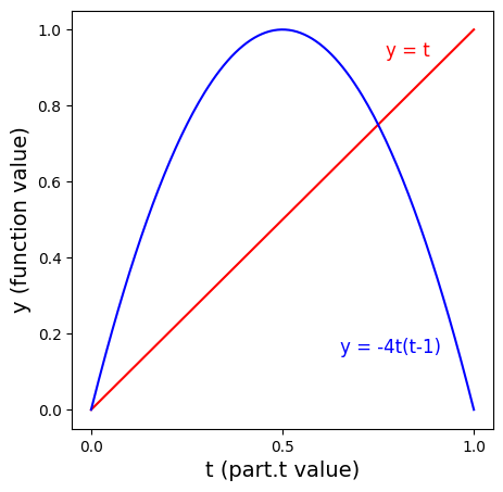
The parabola is 0 at t = 0 and t = 1 and reaches a peak of 1 at t = 0.5. We translate this computation to Lua, with part.t taking the place of t, and save the result to an extra variable shape:
local shape = -4 * part.t * (part.t - 1) -- shaping part.t into a parabola with peak at 0.5
Then we use shape as one additional term in the velocity computation for X and Y:
local shape = -4 * part.t * (part.t - 1)
part.vel.x = -sin(t) * radVel * shape
part.vel.y = -cos(t) * radVel * shape
This should give us a helix that gets fatter in the middle and slims out at both “ends”, following the shape of the parabola:part.vel.x = -sin(t) * radVel * shape
part.vel.y = -cos(t) * radVel * shape
By using this general approach of controlling velocity via part.t, you can create many more intricate curves that the particles will follow. In the repository of module templates, there is an example (trefoil.lua) for a colorful trefoil knot curve:
Okay, I’m nerding out now and I should stop. Hopefully, the idea of shaping particle trajectories by using part.t and various mathematical formulas around it is comprehensible to you, at least in principle. You just need to know what mathematical calculations to apply to part.t to get your desired shape, which depending on your expertise in maths, can get tricky. For now though, we will leave behind the topic of mathematically driven particle motion, as fascinating as it is. If it’s something that you want to pursue further, a more thorough deep-dive into this subject will come in one of the later chapters.
Particle sizeCust and colCust
When it comes to the particle size and color properties, there are respective _Start, _End and _Cust variants for them. All the way back in Chapter 1, when we learned about about these properties in context of init functions, I said that only the _Start and _End variants are important in init, while the _Cust variants are only useful in update functions. Since update functions are now our topic of interest, it’s time to cover the _Cust variants as well._Start and _End property variants (for size and color) are used in init functions to indicate the initial and final values (respectively) of a particle property. The particle’s current size (we can refer to it as “part.sizeNow”, but of course this field doesn’t actually exist!) would be somewhere between part.sizeStart and part.sizeEnd, depending on the age of the particle. Curiously, the t-parameter of a particle (in the 0 to 1 range) also comes into play here, behind the scenes. It’s involved in determining the current size from the Start and End values. The formula for it, carried out inside the plugin, resembles something like this:
part.sizeNow = part.sizeStart * (1 - part.t) + part.sizeEnd * part.t
Side note: the general formula that looks like this:
c = a * (1 - t) + b * t
where a and b are arbitrary values to be blended together, and t is between 0 and 1, is known as a linear interpolation, or a lerp. I am bringing your attention to it, because it’s very useful and we will be using it quite often later on, in the form of the API function lerp().This idea of linear interpolation also applies to how part.colStart and part.colEnd behave. The current color of the particle is linearly blended (separately for each color channel) between these two colors, depending on how old the particle is (also factoring in the part.colFadeTime property, if it was set to a non-default value).
What are the _Cust fields for, then? If we do not make any assigments to them, they simply carry the current blended values of the properties they represent (the ficticious “part.sizeNow” and “part.colNow”). However, when you assign some value, e.g. a size to the particle’s part.sizeCust field or a color to the part.colCust field, this will result in overriding the blended size (or color), for a single frame.
Importantly, this overriding of the _Cust value is valid for a duration of only one frame. The particle system will reset the size (or color) with the re-calculated blended value for the next frame again. This is why assigning to these _Cust variants in init functions serves no purpose, as we need to override the blended values from the particle system on every frame to see the result. Fortunately, this job can be perfectly accomplished by the update function, since its very purpose is to change particle properties on every single frame.
Modifying sizeCust
You can combine the knowledge regarding the t-parameter and part.sizeCust to make the size of a particle change dynamically, depending on the part.t value. For example, making the particle repeatedly grow and shrink with our beloved sin() function.Dealing with part.sizeCust is rather straightforward, you just assign the size values, provided by your custom formula, in the update function. Below is a simple example:
local function sizeUpdate(part)
local cycles = 10 -- var for determining number of grow/shrink cycles
local t = part.t * PI_TWO * cycles -- pre-multiply the t-parameter and save it in a var
part.sizeCust = sin(t) * 100 + 150 -- oscillate size between 50 and 250
end
We first create a helper variable cycles, which counts how many grow/shrink cycles the particle is meant to do over its lifespan. Then, we’re taking part.t, multiplying it by PI_TWO and cycles, and saving it to local t. We then take the rescaled t value and pass it into sin(). The result of sin(t) is then multiplied by 100. This should result in value between [-100, 100]. Obviously, particles cannot have negative size value though, so as a final correction, we add 150 on top, shifting the oscillation range from [-100, 100] to [50, 250]. We assign this final result to part.sizeCust. This should result in the particles smoothly oscillating in size, in approximately 10 cycles, between 50 and 250.local cycles = 10 -- var for determining number of grow/shrink cycles
local t = part.t * PI_TWO * cycles -- pre-multiply the t-parameter and save it in a var
part.sizeCust = sin(t) * 100 + 150 -- oscillate size between 50 and 250
end
Side note: what would the difference be if we used the value of getGameTick() instead of part.t as the input for sin()? Well, since the game tick is a uniform value, not unique to each particle like part.t, all the particles would be synchronized, growing / shrinking simultaneously. Conversely, part.t represents the individual age of each particle, so they will grow and shrink independently of each other. Certainly, we could have used getGameTick() to get a different result, it depends on what we’re going for.
We needed to mathematically transform the raw output of sin(t), to get values that do not dive into negative numbers and at the same time are in a sensible range, to take a noticeable effect on part.sizeCust. This formula ended up being sin(t) * 100 + 150, which is not too complicated. However, figuring out the correct math each time to obtain a desired min/max range feels cumbersome. Is there an easier way? Yes!
The remap() function
When it comes to moving a value from one range to another, like we just witnessed in the last example:- scaling part.t from [0, 1] to [0, 20π];
- moving the output range of sin(t) from [-1, 1] over to [50, 250]
remap(x, oldMin, oldMax, newMin, newMax) -- remaps argument "x" from [oldMin, oldMax] to [newMin, newMax]
To call this function, we must specify the x value which will be remapped, the original min-max range of the x value with the pair oldMin, oldMax, then finally the new range, via newMin, newMax.We can do two remappings. The first one, to scale part.t by 2π * cycles:
local t = remap(part.t, 0, 1, 0, PI_TWO * cycles) -- remap part.t from [0, 1] to [0, 2π * cycles]
and then the second one, take the output of sin(t) from [-1, 1] and remap it to [50, 250]:
part.sizeCust = remap(sin(t), -1, 1, 50, 250) -- remap sin(t) from [-1, 1] to [50, 250]
These remap function calls effectively will do the same thing as the mathematical calculations from before, but I think it simplifies obtaining the correct values quite a bit, because you do not need to think about the exact mathematical formula to get your expected result. The only caveat is knowing what the original range of the remapped x value is. As an example, for part.t it’s [0, 1], while for the outputs of trigonometric functions sin() and cos(), the range is [-1, 1]. These become the oldMin, oldMax values, which you are remapping to newMin, newMax.The remap() function serves as an alternative to the previously mentioned function clamp(). The difference is that clamping sets hard boundaries that the x values must fit into, whereas remapping attempts to make the x source value range smoothly fit into the [newMin, newMax] range (thus you must provide information about the [oldMin, oldMax] of the source value). Be aware that the remap() also clamps the x input to fit between [oldMin, oldMax]!
Modifying colCust
Changing particle size on the fly is really neat, but changing particle colors is even cooler! Similarly to the part.sizeCust field, part.colCust allows to override the RGB color values of a particle dynamically in the update function. I will show how we can modify part.colCust by using yet another great function from the API, createColorHSV().HSV Color Space
The function createColorHSV() returs a ColorRGB object. Unlike the ordinary createColor() function, it does not take values for the Red, Green and Blue channels. Instead, it takes arguments of Hue, Saturation and Value, according to the HSV color model. The HSV model works differently than the RGB color model. Instead of specifying the exact amounts of primary colors (Red, Green, Blue) that constitute the final color, in HSV, the color is represented as a combination of Hue, Saturation and Value.- Hue is an angle, expressed in degrees (miraculously, not radians!) between 0 and 360, representing a color wheel smoothly blending hues of red, orange, yellow, green, blue, magenta/purple and back to red again. Conventionally, Hue = 0 corresponds to red and begins the color wheel.
- Saturation describes how saturated the color is. At Saturation 0, the color is either white, black or some shade of grey, with no identifiable hue (the Hue value does not matter now, since it has no influence at Saturation = 0). All values of Saturation above 0 have an identifiable hue. The full Saturation is at 1, which indicates no “greyness” in the color.
- Value describes how dark or bright the color is. As with Saturation, the range of Value is between 0 and 1. At 0, the color is pitch black, RGB(0, 0, 0). Neither Hue nor Saturation influence the color at Value = 0. At Value = 1, the color has no “darkness”. What this means depends further on the Saturation value. At Saturation = 1 and Value = 1, the color is fully saturated. At Saturation = 0 and Value = 1, the color becomes fully white, RGB(255, 255, 255). At middle saturation (around 0.5) and Value = 1 the color becomes a pastel shade, more biased towards white. At full Saturation = 1 and a intermediate Value (around 0.5) the color becomes a darker shade, more biased towards black. No Saturation with an intermediate Value is some shade of gray.
This HSV model of colors has some interesting implications. The Hue value, seen as an angle from 0 to 360 degrees, represents a continuous loop through the color spectrum. This suggests that it should be possible to cycle through it seamlessly. That’s exactly what we will be doing, in the following example involving part.colCust:
local function colorUpdate(part)
-- some code for particle motion can be here
local hue = getGameTick() -- game tick value is interpreted as angle for hue
local sat = 1.0
local val = 1.0
part.colCust = createColorHSV(hue, sat, val)
end
The particles will oscillate between different hues as the game tick counter increases.-- some code for particle motion can be here
local hue = getGameTick() -- game tick value is interpreted as angle for hue
local sat = 1.0
local val = 1.0
part.colCust = createColorHSV(hue, sat, val)
end
They are oscillating uniformly, though, all at the same time, since game tick values are uniform for each particle. We can also obtain a “spectrum scrolling” effect by including part.t in the picture. We rework the formula for hue, first multiplying part.t by 180, then adding getGameTick() on top of that:
local hue = part.t * 180 + getGameTick() -- individual particle delay via part.t
By how much we multiply part.t, we control the difference between the starting hue and ending hue in the color scroll. You may also do without the getGameTick() value (making it entirely depend on part.t), or even use some other inputs for createColorHSV(). Have some fun with it and try out different combinations!
Modifying RGB values individually
In the above example, we were assigning colors directly to the field part.colCust as a whole. Nothing is preventing us from modifying the RGB color components of colCust individually, though. We can then control the value for each color channel with a separate formula. I just want to re-emphasize that the color fields accept only integers from the 0-255 range per each channel. Thus, we must clamp or remap whatever result we get, e.g. from a function like sin(), to [0, 255].
local function rgbUpdate(part)
-- some code for particle motion can be here
local t = part.t * 3 * PI
local d = PI * 2 / 3
local sinr = sin(t)
local sing = sin(t + d)
local sinb = sin(t + 2*d)
part.colCust.r = remap(sinr, -1, 1, 0, 255)
part.colCust.g = remap(sing, -1, 1, 0, 255)
part.colCust.b = remap(sinb, -1, 1, 0, 255)
end
-- some code for particle motion can be here
local t = part.t * 3 * PI
local d = PI * 2 / 3
local sinr = sin(t)
local sing = sin(t + d)
local sinb = sin(t + 2*d)
part.colCust.r = remap(sinr, -1, 1, 0, 255)
part.colCust.g = remap(sing, -1, 1, 0, 255)
part.colCust.b = remap(sinb, -1, 1, 0, 255)
end
Fun stuff! Feel free to play around and see what curious color patterns you can come up with by using this technique.
As this chapter is quite long already, I’ve decided to split it in half here, since this is a good point to pause. The next half continues with topics such as particle function and particles that spawn other particles. That’s where update functions can really shine and show their true power! Take a break if you need one and I’ll see you there!
| « PREV | NEXT » |